Connect 4 Algorithm
In order for the robot to play competitively against a human, a minimax game algorithm is used to choose the best move in response to the human player. The algorithm’s ‘game loop’ is implemented inside the main file, but for general tidiness all of the algorithm functions are stored in a separate file.
Setup Functions
Create a numpy array of zeroes to represent the Connect 4 board. This will be populated with numbered pieces throughout the game.
def create_board():
    board = np.zeros((ROW_COUNT, COLUMN_COUNT))
    return board
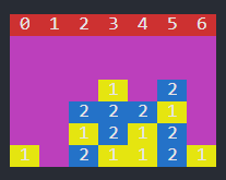
Set up the board to print out in the terminal in a way that makes it visually easy to play with the computer.
def pretty_print_board(board):
    flipped_board = np.flipud(board)

    print("\033[0;37;41m 0 \033[0;37;41m 1 \033[0;37;41m 2 \033[0;37;41m 3 \033[0;37;41m 4 \033[0;37;41m 5 \033[0;37;41m 6 \033[0m")
    for i in flipped_board:
        row_str = ""

        for j in i:
            if j == 1:
                #print(yellow)
                row_str +="\033[0;37;43m 1 "
            elif j ==2:
                row_str +="\033[0;37;44m 2 "
            else:
                #print black
                row_str +="\033[0;37;45m   "

        print(row_str+"\033[0m")
Note
Due to restrictions on the version of numpy, np.flipud(board) was used instead of the most up to date version: np.flip(board).
If you are using the most up to date version of numpy, you can update this function (although it will not break if you do not - numpy has reasonably good backwards-compatibility).
Warning
It’s important to understand that the algorithm fills the board from the top down. In real life, the board fills up from the bottom. np.flipud(board) flips the board around a horizontal axis, making it the correct visual orientation for Connect 4.
In future, for clarity and ease of understanding, the placement of the pieces within the board will be referred to in the same way that it would happen in real life (bottom up).
There are 4 functions that are used when placing a piece on the board.
- To get all locations in the board that could contain a piece (i.e. have not yet been filled):
def get_valid_locations(board):
    valid_locations = []
    for col in range(COLUMN_COUNT):
        if is_valid_location(board, col):
            valid_locations.append(col)
    return valid_locations
- To check if there is a valid location in the chosen column:
def is_valid_location(board, col):
    return board[ROW_COUNT - 1][col] == 0
- To check which row the piece can be placed into (i.e. the next available open row):
def get_next_open_row(board, col):
    for r in range(ROW_COUNT):
        if board[r][col] == 0:
            return r
Note
This function serves as virtual ‘gravity’. Instead of placing a piece anywhere in the column, by getting only the next open row, piece placement is restricted to the next available slot from the bottom of the board, as would happen in real life. This also means that the only input that is required is now the column (the row is automatically found and assigned).
- Finally, to place a piece in the next available row, in the chosen column:
def drop_piece(board, row, col, piece):
    board[row][col] = piece
Analysis Functions
When the human player (Player 1) has made a move, the drop_piece function will update the numpy array board with a number 1 in the specified position. In order for the game algorithm (Player 2) to choose the best move to play in response, it has to understand and analyse the current board state. This is done using a ‘windowing’ technique.
In the following function, horizontal, vertical, positive (upward sloping) and negative (downward sloping) diagonal windows are created. These windows are then used to scan all possible 4-piece sections of the board, and evaluate (score) each window based on its contents.
This evaluation is performed separately by the evaluate_window function, which is called within the score_position function, and explained in further detail below.
def score_position(board, piece):
    score = 0

    # Score centre column
    centre_array = [int(i) for i in list(board[:, COLUMN_COUNT // 2])]
    centre_count = centre_array.count(piece)
    score += centre_count * 3

    # Score horizontal positions
    for r in range(ROW_COUNT):
        row_array = [int(i) for i in list(board[r, :])]
        for c in range(COLUMN_COUNT - 3):
            # Create a horizontal window of 4
            window = row_array[c:c + WINDOW_LENGTH]
            score += evaluate_window(window, piece)

    # Score vertical positions
    for c in range(COLUMN_COUNT):
        col_array = [int(i) for i in list(board[:, c])]
        for r in range(ROW_COUNT - 3):
            # Create a vertical window of 4
            window = col_array[r:r + WINDOW_LENGTH]
            score += evaluate_window(window, piece)

    # Score positive diagonals
    for r in range(ROW_COUNT - 3):
        for c in range(COLUMN_COUNT - 3):
            # Create a positive diagonal window of 4
            window = [board[r + i][c + i] for i in range(WINDOW_LENGTH)]
            score += evaluate_window(window, piece)

    # Score negative diagonals
    for r in range(ROW_COUNT - 3):
        for c in range(COLUMN_COUNT - 3):
            # Create a negative diagonal window of 4
            window = [board[r + 3 - i][c + i] for i in range(WINDOW_LENGTH)]
            score += evaluate_window(window, piece)

    return score
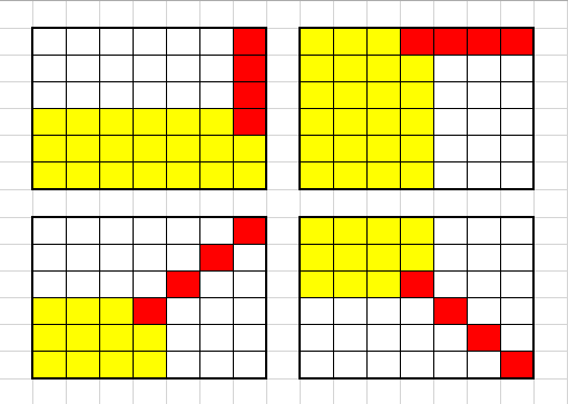
The figure below shows the scanning range for this score_position function. It is unnecessary to use every index of the board as a starting position for a scanning window, because in many positions some windows would then extend over the sides of the board.
As a result, there are only 69 positions in which the scanning window needs to be deployed. The yellow highlight shows the applicable scanning range, and the red squares are an example of a scanning window in the maximum required position.
The evaluate_window function is called in the last line of each scoring block. The output of this evaluation function (a numerical score value) is stored in the score variable, which is updated every time a higher score is found.
When the scanning is complete, the window with the best score is passed to the game algorithm to play a move. Note that this scoring mechanism is required, but the minimax function, which will be explained in further detail, makes some elements of this function much less important.
In any given scanning position, the contents of that window are evaluated for ‘strength’, e.g. a window that contains 3 consecutive pieces from the same player is a ‘strong’ state, and has a higher score. This means that the algorithm is more likely to try and create board states that are ‘strong’ - i.e. prioritise connecting 3 pieces together, rather than connecting 2.
def evaluate_window(window, piece):
    score = 0
    # Switch scoring based on turn
    opp_piece = PLAYER_PIECE
    if piece == PLAYER_PIECE:
        opp_piece = BOT_PIECE

    # Prioritise a winning move
    # Minimax makes this less important
    if window.count(piece) == 4:
        score += 100
    # Make connecting 3 second priority
    elif window.count(piece) == 3 and window.count(EMPTY) == 1:
        score += 5
    # Make connecting 2 third priority
    elif window.count(piece) == 2 and window.count(EMPTY) == 2:
        score += 2
    # Prioritise blocking an opponent's winning move (but not over bot winning)
    # Minimax makes this less important
    if window.count(opp_piece) == 3 and window.count(EMPTY) == 1:
        score -= 4

    return score
The final element of the analysis is a ‘special case’ variation of the score_position function. When 4 pieces are joined together, this signifies the game has been won.
After every move, the board needs to be scanned by both the score_position function, and also the winning_move function, which will exit out of the game loop if it sees a winning move.
def winning_move(board, piece):
    # Check valid horizontal locations for win
    for c in range(COLUMN_COUNT - 3):
        for r in range(ROW_COUNT):
            if board[r][c] == piece and board[r][c + 1] == piece and board[r][c + 2] == piece and board[r][c + 3] == piece:
                return True

    # Check valid vertical locations for win
    for c in range(COLUMN_COUNT):
        for r in range(ROW_COUNT - 3):
            if board[r][c] == piece and board[r + 1][c] == piece and board[r + 2][c] == piece and board[r + 3][c] == piece:
                return True

    # Check valid positive diagonal locations for win
    for c in range(COLUMN_COUNT - 3):
        for r in range(ROW_COUNT - 3):
            if board[r][c] == piece and board[r + 1][c + 1] == piece and board[r + 2][c + 2] == piece and board[r + 3][c + 3] == piece:
                return True

    # check valid negative diagonal locations for win
    for c in range(COLUMN_COUNT - 3):
        for r in range(3, ROW_COUNT):
            if board[r][c] == piece and board[r - 1][c + 1] == piece and board[r - 2][c + 2] == piece and board[r - 3][c + 3] == piece:
                return True
Algorithm
The algorithm chosen to play Connect 4 is the minimax algorithm. Minimax is a backtracking algorithm which is commonly used in decision-making and game theory to find the optimal move for a player. This makes it a perfect choice for two-player, turn-based games.
In the minimax algorithm, the two players are the maximiser and minimiser. The maximiser is trying to get the highest score possible, and the minimiser is trying to get the lowest score possible.
The best / worst scores are calculated by the evaluate_window function, and stored in the score variable, described in the previous section.
At the start of every turn, minimax will scan the board’s remaining valid locations and calculate all possible moves, before backtracking and choosing the optimal move for that turn. This will be either the best or worst move, depending on whether it is the maximiser or minimiser’s turn. The assumption is that minimax (maximiser) can play optimally, as long as the human player (minimiser) also plays optimally. This will not always be the case, but does not lead to significant gameplay problems.
Before implementing the minimax algorithm, the two game-terminating states need to be defined as terminal nodes. If there is a winning move from either player, or if the board fills up without a win (leading to a draw), the game will end.
def is_terminal_node(board):
    return winning_move(board, PLAYER_PIECE) or winning_move(board, BOT_PIECE) or len(get_valid_locations(board)) == 0
The minimax algorithm for the Connect 4 game is implemented below.
def minimax(board, depth, alpha, beta, maximisingPlayer):
    valid_locations = get_valid_locations(board)

    is_terminal = is_terminal_node(board)
    if depth == 0 or is_terminal:
        if is_terminal:
            # Weight the bot winning really high
            if winning_move(board, BOT_PIECE):
                return (None, 9999999)
            # Weight the human winning really low
            elif winning_move(board, PLAYER_PIECE):
                return (None, -9999999)
            else:  # No more valid moves
                return (None, 0)
        # Return the bot's score
        else:
            return (None, score_position(board, BOT_PIECE))

    if maximisingPlayer:
        value = -9999999
        # Randomise column to start
        column = random.choice(valid_locations)
        for col in valid_locations:
            row = get_next_open_row(board, col)
            # Create a copy of the board
            b_copy = board.copy()
            # Drop a piece in the temporary board and record score
            drop_piece(b_copy, row, col, BOT_PIECE)
            new_score = minimax(b_copy, depth - 1, alpha, beta, False)[1]
            if new_score > value:
                value = new_score
                # Make 'column' the best scoring column we can get
                column = col
            alpha = max(alpha, value)
            if alpha >= beta:
                break
        return column, value

    else:  # Minimising player
        value = 9999999
        # Randomise column to start
        column = random.choice(valid_locations)
        for col in valid_locations:
            row = get_next_open_row(board, col)
            # Create a copy of the board
            b_copy = board.copy()
            # Drop a piece in the temporary board and record score
            drop_piece(b_copy, row, col, PLAYER_PIECE)
            new_score = minimax(b_copy, depth - 1, alpha, beta, True)[1]
            if new_score < value:
                value = new_score
                # Make 'column' the best scoring column we can get
                column = col
            beta = min(beta, value)
            if alpha >= beta:
                break
        return column, value
Note
The implementation of this minimax algorithm also contains Alpha-Beta pruning. There is no point following a decision-tree branch any further if the initial move scores less optimally than an alternative move that has already been discovered. Alpha-Beta pruning works to ‘prune’ away these branches, leaving a much smaller, more optimised decision tree.
This technique is used to reduce the time complexity of the algorithm, which in this context is important, as there are many other parts of the game loop that are time consuming (e.g. Motion Planning). The game algorithm can now run reliably in under 500ms, even when looking 4 moves into the future.
Limitations / Improvements
There are some key limitations to the algorithm, but they did not need to be directly addressed as they were outside the scope for this project.
- Lack of scalability
Due to the hard-coded nature of the scanning procedure, the board size, the number of connected pieces required to win, and the scanning window size cannot be changed without causing major errors. This would not be particuarly difficult to fix, but would require a different, more adaptive scanning structure and further definition of static variables.
- Incomplete win structure
During stress testing, it became clear that the algorithm would not make a winning move if there were two or more possible winning moves available. This is presumably because it could not decide between equally weighted branches, and therefore made the ‘next best’ move. This problem did not impact the algorithm’s success rate, however, because as soon as the human player filled one of the possible winning spaces, the algorithm would win the game using the other.